Geometric Derivation of Euler-Lagrange Equation
Statement
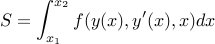
Given a functional  :
:
Euler-Lagrange says that the function  at a stationary point of the
functional obeys:
at a stationary point of the
functional obeys:
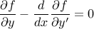
Where  .
.
This result is often proven using integration by parts – but the equation expresses a local condition, and should be derivable using local reasoning.
We will explore an alternate derivation below.
Motivating Example
Physical systems in stable equilibrium will move to a configuration that
locally minimizes their potential energy.
For example, consider a chain draped over two pulleys (at height  , separated
by distance
, separated
by distance  ),
with excess chain resting on the ground.
),
with excess chain resting on the ground.
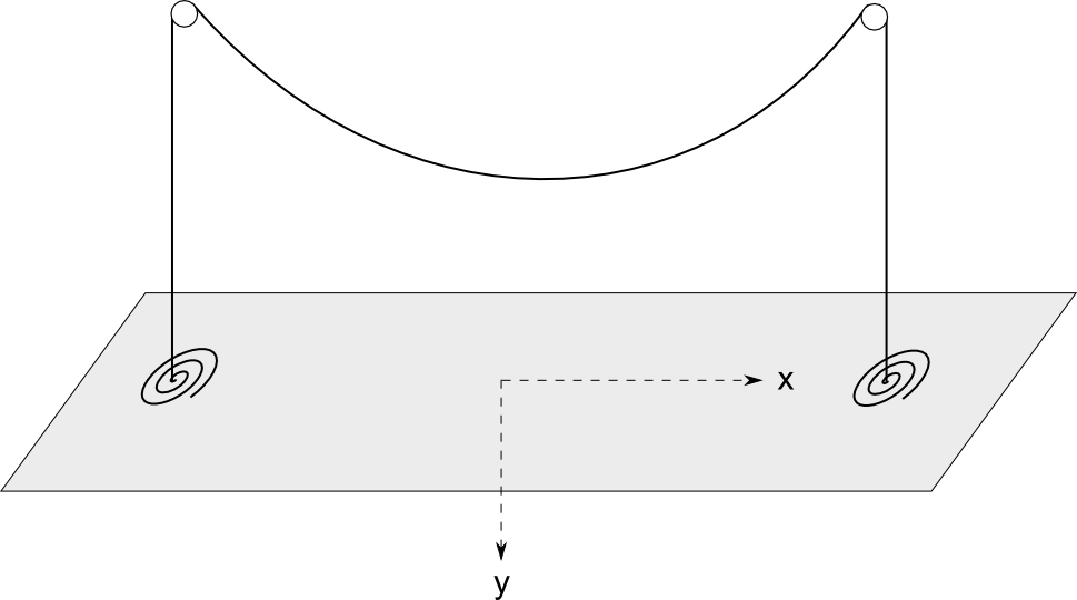 |
The chain will take a shape between the two pulleys that minimizes its gravitational potential energy. The space is interesting: If the chain is taut, then it will be high above the ground, and have high energy. If the chain is very saggy, it will pull up lots of chain from the ground, and have high energy. In between is the optimal shape.
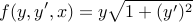
The potential energy of a given shape of the chain between the pulleys is:
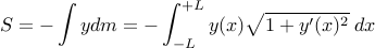
We have integrated only along the section between the pulleys, because
we can define  at ground level, and ignore constants (the energy of the
chain dangling outside the pulleys) and constant factors (
at ground level, and ignore constants (the energy of the
chain dangling outside the pulleys) and constant factors ( ).
).
Now we want to find the function that minimizes
(subject to the boundary conditions 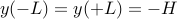 ).
).
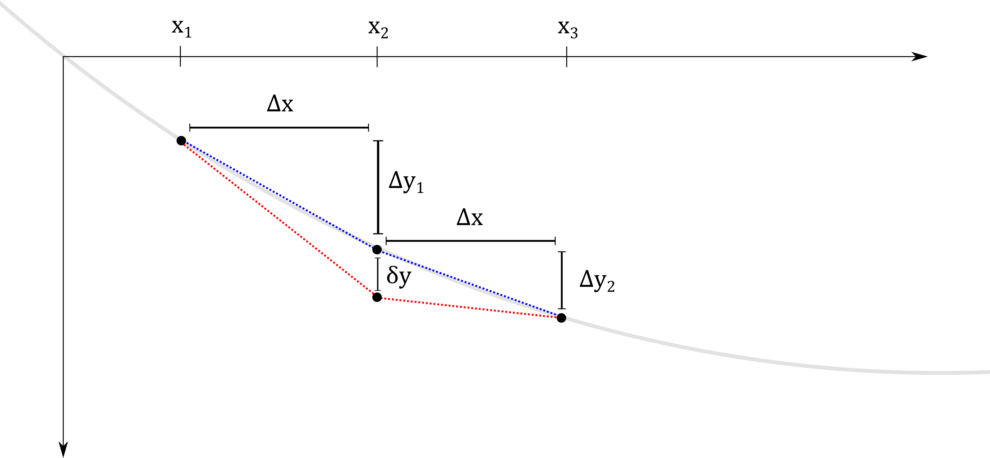
Geometric Derivation
For  to be a stationary point of , small perturbations to the function
must not alter the value of (to first order). So consider an
infinitesimal segment of (grey), discretized around
to be a stationary point of , small perturbations to the function
must not alter the value of (to first order). So consider an
infinitesimal segment of (grey), discretized around  .
We will consider perturbing at by an amount
.
We will consider perturbing at by an amount  (changing
from the blue –> red), and examine its effect
(changing
from the blue –> red), and examine its effect  on .
on .
 |
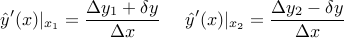
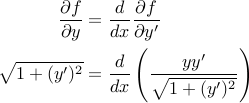
Recall: 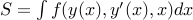
Perturbing this point affects  in two ways:
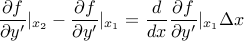
It alters the value of
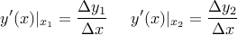
at .It alters the derivatives
 around .
The first contribution is simply:

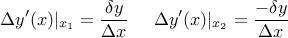
The second contribution is in two parts: increasing the derivative on the left, and decreasing the derivative on the right. Based on the figure, we have (before perturbation):
And after perturbation:
So the change in derivatives is:
This affects by an amount:
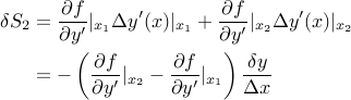
Since  , we can write:
So finally, the effect of changing the derivatives is:
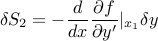
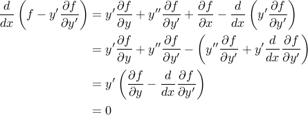
And the net effect of perturbing the point is:
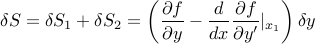
So clearly, requiring  for small perturbations
anywhere along the function implies the Euler-Lagrange equation:
for small perturbations
anywhere along the function implies the Euler-Lagrange equation:
And now both terms have meaning:
 : The amount small perturbations affect
by directly changing the value .
: The amount small perturbations affect
by directly changing the value . : The net amount perturbations
affect by changing the derivatives in the neighborhood of
: The net amount perturbations
affect by changing the derivatives in the neighborhood of  .
(the derivative to the left increases, and to the right decreases – so
the net effect depends on how
.
(the derivative to the left increases, and to the right decreases – so
the net effect depends on how  changes over
the span
changes over
the span  ).
).
At a stationary point, these effects must exactly cancel.
Final Comments
For completeness, we derive the solution to the example, and extend it to the case of a fixed-length chain.
Solution
In this case:
Applying Euler-Lagrange directly, we find:
We could solve this, but the simpler approach is to use a theorem:
Thm: If  , then
  is a constant.
Proof:
Where the last step is applying the original form of the Euler-Lagrange equation.
Since our particular  is independent of , we can apply this
theorem:
is independent of , we can apply this
theorem:
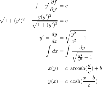
For constants  chosen to satisfy boundary conditions. This gives us the
familiar catenary curve.
chosen to satisfy boundary conditions. This gives us the
familiar catenary curve.
Extension
We know the catenary is also the shape formed if we hang a fixed-length chain between two fixed endpoints. This is no coincidence.
The fixed-length chain problem is a constrained minimization problem,
with the same potential energy functional , but the additional constraint that the
arclength of is some specified constant.
Specify constrained problems by  – separation distance and chain arclength.
And unconstrained problems by  – separation distance and height.
We will show that the solution to this problem is also a catenary, by showing that:
Theorem: For a given constrained-problem , there is a
corresponding unconstrained-problem that contains the
constrained-problem as a sub-problem. Therefore the constrained problem must
also be a catenary.
Lemma: For any  , we can always find some unconstrained configuration
such that the length of chain between
, we can always find some unconstrained configuration
such that the length of chain between  and
and  is exactly
  .
.
Proof: Refer to the family of unconstrained solutions we found.
With centered choice of coordinates,  , and the family takes the form:
The boundary condition  determines the parameter
  .
Now, clearly the arclength between and is a monotone
decreasing function of , with extremes at
.
Now, clearly the arclength between and is a monotone
decreasing function of , with extremes at  and
and  .
(eg, for
.
(eg, for  , the arclength turns out to be
  )
)
So any value of in this range is achievable for some  – and further,
there is some that gives rise to this
(in particular,
– and further,
there is some that gives rise to this
(in particular,  works).
Result: Now, given a constrained-problem ,
construct an unconstrained-problem  such that
the length of chain between
such that
the length of chain between  and
and  is exactly
  . (which Lemma
guarentees we are able to do). Over this span, the unconstrained problem is
identical to the constrained problem: arclength , and endpoints separated by
. If one situation's optimal-solution (say A)
had lower potential energy (over the span) than the
other (B), then B could assume the form of A over the span, without violating
any constraints but resulting in lower energy. Contradiction of optimality, so
both problems must have identical solutions over the span – and the constrained
optimal solution is also a catenary.
. (which Lemma
guarentees we are able to do). Over this span, the unconstrained problem is
identical to the constrained problem: arclength , and endpoints separated by
. If one situation's optimal-solution (say A)
had lower potential energy (over the span) than the
other (B), then B could assume the form of A over the span, without violating
any constraints but resulting in lower energy. Contradiction of optimality, so
both problems must have identical solutions over the span – and the constrained
optimal solution is also a catenary.
So we have also derived the solution to the constrained problem. (no Lagrange multipliers necessary!)